Calculating Antenna Array Performance Envelope using Aperture Projection

This is a demonstration using the aperture projection function in the context of a conformal antenna array mounted upon an unmanned aerial vehicle.

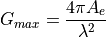
Aperture Projection as a technique is based upon Hannan’s formulation of the gain of an aperture based upon its surface area and the freuqency of interest. This is defined in terms of the maximum gain , the effective area of the aperture , and the wavelength of interest .

While this has been in common use since the 70s, as a formula it is limited to planar surfaces, and only providing the maximum gain in the boresight direction for that surface.

Aperture projection as a function is based upon the rectilinear projection of the aperture into the farfield. This can then be used with Hannan’s formula to predict the maximum achievable directivity for all farfield directions of interest.

As this method is built into a raytracing environment, the maximum performance for an aperture on any platform can also be predicted using the lyceanem.models.frequency_domain.aperture_projection() function.

import numpy as np
import open3d as o3d
import copy

Setting Farfield Resolution and Wavelength

LyceanEM uses Elevation and Azimuth to record spherical coordinates, ranging from -180 to 180 degrees in azimuth, and from -90 to 90 degrees in elevation. In order to launch the aperture projection function, the resolution in both azimuth and elevation is requried. In order to ensure a fast example, 37 points have been used here for both, giving a total of 1369 farfield points.

The wavelength of interest is also an important variable for antenna array analysis, so we set it now for 10GHz, an X band aperture.

az_res = 37
elev_res = 37
wavelength = 3e8 / 10e9

Geometries

In order to make things easy to start, an example geometry has been included within LyceanEM for a UAV, and the open3d trianglemesh structures can be accessed by importing the data subpackage

import lyceanem.tests.reflectordata as data

body, array, _ = data.exampleUAV(10e9)

# visualise UAV and Array
o3d.visualization.draw_geometries([body, array])

# .. image:: ../_static/open3d_structure.png

# crop the inner surface of the array trianglemesh (not strictly required, as the UAV main body provides blocking to
# the hidden surfaces, but correctly an aperture will only have an outer face.
surface_array = copy.deepcopy(array)
surface_array.triangles = o3d.utility.Vector3iVector(
    np.asarray(array.triangles)[: len(array.triangles) // 2, :]
)
surface_array.triangle_normals = o3d.utility.Vector3dVector(
    np.asarray(array.triangle_normals)[: len(array.triangle_normals) // 2, :]
)

Structures

LyceanEM uses a class named ‘structures’ to store and maniuplate joined 3D solids. Currently all that is implemented is the class itself, and methods to allow translation and rotation of the trianglemesh solids. A structure can be passed to the models to provide the environment to be considered as blockers. structures are created by calling the class, and passing it a list of the open3d trianglemesh structures to be added.

from lyceanem.base_classes import structures

blockers = structures([body])

Aperture Projection

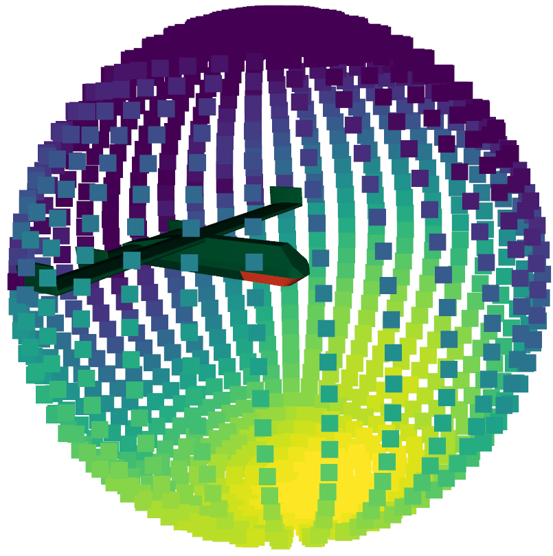
Aperture Projection is imported from the frequency domain models, requiring the aperture of interest, wavelength to be considered, and the azimuth and elevation ranges. The function then returns the directivity envelope as a numpy array of floats, and an open3d point cloud with points and colors corresponding to the directivity envelope of the provided aperture, scaling from yellow at maximum to dark purple at minimum.

from lyceanem.models.frequency_domain import aperture_projection

directivity_envelope, pcd = aperture_projection(
    surface_array,
    environment=blockers,
    wavelength=wavelength,
    az_range=np.linspace(-180.0, 180.0, az_res),
    elev_range=np.linspace(-90.0, 90.0, elev_res),
)

Open3D Visualisation

The resultant maximum directivity envelope is provided as both a numpy array of directivities for each angle, but also as an open3d point cloud. This allows easy visualisation using open3d.visualization.draw_geometries(). %%

o3d.visualization.draw_geometries([body, surface_array, pcd])

# Maximum Directivity
print(
    "Maximum Directivity of {:3.1f} dBi".format(
        np.max(10 * np.log10(directivity_envelope))
    )
)

Maximum Directivity of 18.5 dBi

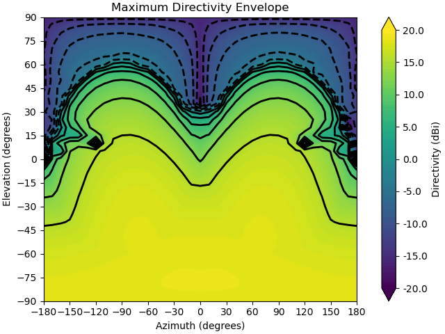
Plotting the Output

While the open3d visualisation is very intuitive for examining the results of the aperture projection, it is difficult to consider the full 3D space, and cannot be included in documentation in this form. However, matplotlib can be used to generate contour plots with 3dB contours to give a more systematic understanding of the resultant maximum directivity envelope.

import matplotlib.pyplot as plt

# set directivity limits on the closest multiple of 5
plot_max = ((np.ceil(np.nanmax(10 * np.log10(directivity_envelope))) // 5.0) + 1) * 5
azmesh, elevmesh = np.meshgrid(
    np.linspace(-180.0, 180.0, az_res), np.linspace(-90, 90, elev_res)
)
fig, ax = plt.subplots(constrained_layout=True)
origin = "lower"

levels = np.linspace(plot_max - 40, plot_max, 81)
CS = ax.contourf(
    azmesh,
    elevmesh,
    10 * np.log10(directivity_envelope),
    levels,
    origin=origin,
    extend="both",
)
cbar = fig.colorbar(CS)
cbar.ax.set_ylabel("Directivity (dBi)")
cbar.set_ticks(np.linspace(plot_max - 40, plot_max, 9))
cbar.ax.set_yticklabels(np.linspace(plot_max - 40, plot_max, 9).astype("str"))
levels2 = np.linspace(
    np.nanmax(10 * np.log10(directivity_envelope)) - 60,
    np.nanmax(10 * np.log10(directivity_envelope)),
    21,
)
CS4 = ax.contour(
    azmesh,
    elevmesh,
    10 * np.log10(directivity_envelope),
    levels2,
    colors=("k",),
    linewidths=(2,),
    origin=origin,
)
ax.set_ylim(-90, 90)
ax.set_xlim(-180.0, 180)
ax.set_xticks(np.linspace(-180, 180, 13))
ax.set_yticks(np.linspace(-90, 90, 13))
ax.set_xlabel("Azimuth (degrees)")
ax.set_ylabel("Elevation (degrees)")
ax.set_title("Maximum Directivity Envelope")
fig.show()