Modelling a Physical Channel in the Frequency Domain

This example uses the frequency domain lyceanem.models.frequency_domain.calculate_scattering() function to predict the scattering parameters for the frequency and environment included in the model. This model allows for a very wide range of antennas and antenna arrays to be considered, but for simplicity only horn antennas will be included in this example. The simplest case would be a single source point and single receive point, rather than an aperture antenna such as a horn.

import numpy as np
import open3d as o3d
import copy

Frequency and Mesh Resolution

freq = np.asarray(15.0e9)
wavelength = 3e8 / freq
mesh_resolution = 0.5 * wavelength

Setup transmitters and receivers

import lyceanem.geometry.targets as TL
import lyceanem.geometry.geometryfunctions as GF

transmit_horn_structure, transmitting_antenna_surface_coords = TL.meshedHorn(
    58e-3, 58e-3, 128e-3, 2e-3, 0.21, mesh_resolution
)
receive_horn_structure, receiving_antenna_surface_coords = TL.meshedHorn(
    58e-3, 58e-3, 128e-3, 2e-3, 0.21, mesh_resolution
)

Position Transmitter

rotate the transmitting antenna to the desired orientation, and then translate to final position. lyceanem.geometryfunctions.open3drotate() allows both the center of rotation to be defined, and ensures the right syntax is used for Open3d, as it was changed from 0.9.0 to 0.10.0 and onwards.

rotation_vector1 = np.radians(np.asarray([90.0, 0.0, 0.0]))
rotation_vector2 = np.radians(np.asarray([0.0, 0.0, -90.0]))
transmit_horn_structure = GF.open3drotate(
    transmit_horn_structure,
    o3d.geometry.TriangleMesh.get_rotation_matrix_from_xyz(rotation_vector1),
)
transmit_horn_structure = GF.open3drotate(
    transmit_horn_structure,
    o3d.geometry.TriangleMesh.get_rotation_matrix_from_xyz(rotation_vector2),
)
transmit_horn_structure.translate(np.asarray([2.695, 0, 0]), relative=True)
transmitting_antenna_surface_coords = GF.open3drotate(
    transmitting_antenna_surface_coords,
    o3d.geometry.TriangleMesh.get_rotation_matrix_from_xyz(rotation_vector1),
)
transmitting_antenna_surface_coords = GF.open3drotate(
    transmitting_antenna_surface_coords,
    o3d.geometry.TriangleMesh.get_rotation_matrix_from_xyz(rotation_vector2),
)
transmitting_antenna_surface_coords.translate(np.asarray([2.695, 0, 0]), relative=True)

Out:

geometry::PointCloud with 36 points.

Position Receiver

rotate the receiving horn to desired orientation and translate to final position.

receive_horn_structure = GF.open3drotate(
    receive_horn_structure,
    o3d.geometry.TriangleMesh.get_rotation_matrix_from_xyz(rotation_vector1),
)
receive_horn_structure.translate(np.asarray([0, 1.427, 0]), relative=True)
receiving_antenna_surface_coords = GF.open3drotate(
    receiving_antenna_surface_coords,
    o3d.geometry.TriangleMesh.get_rotation_matrix_from_xyz(rotation_vector1),
)
receiving_antenna_surface_coords.translate(np.asarray([0, 1.427, 0]), relative=True)

Out:

geometry::PointCloud with 36 points.

Create Scattering Plate

Create a Scattering plate a source of multipath reflections

reflectorplate, scatter_points = TL.meshedReflector(
    0.3, 0.3, 6e-3, wavelength * 0.5, sides="front"
)
position_vector = np.asarray([29e-3, 0.0, 0])
rotation_vector1 = np.radians(np.asarray([0.0, 90.0, 0.0]))
scatter_points = GF.open3drotate(
    scatter_points,
    o3d.geometry.TriangleMesh.get_rotation_matrix_from_xyz(rotation_vector1),
)
reflectorplate = GF.open3drotate(
    reflectorplate,
    o3d.geometry.TriangleMesh.get_rotation_matrix_from_xyz(rotation_vector1),
)
reflectorplate.translate(position_vector, relative=True)
scatter_points.translate(position_vector, relative=True)

Out:

geometry::PointCloud with 900 points.

Specify Reflection Angle

Rotate the scattering plate to the optimum angle for reflection from the transmitting to receiving horn

plate_orientation_angle = 45.0

rotation_vector = np.radians(np.asarray([0.0, 0.0, plate_orientation_angle]))
scatter_points = GF.open3drotate(
    scatter_points,
    o3d.geometry.TriangleMesh.get_rotation_matrix_from_xyz(rotation_vector),
)
reflectorplate = GF.open3drotate(
    reflectorplate,
    o3d.geometry.TriangleMesh.get_rotation_matrix_from_xyz(rotation_vector),
)

from lyceanem.base_classes import structures

blockers = structures([reflectorplate, receive_horn_structure, transmit_horn_structure])

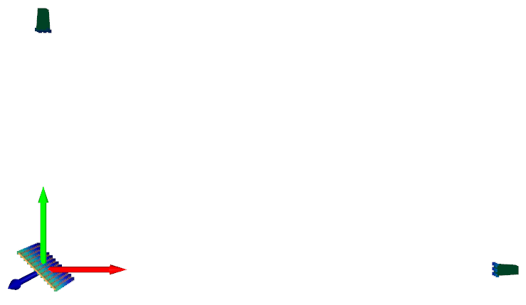
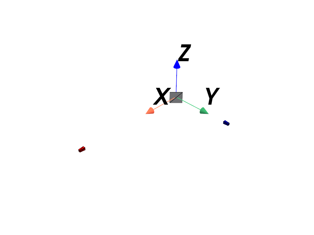
Visualise the Scene Geometry

Use open3d function open3d.visualization.draw_geometries() to visualise the scene and ensure that all the relavent sources and scatter points are correct. Point normal vectors can be displayed by pressing ‘n’ while the window is open.

mesh_frame = o3d.geometry.TriangleMesh.create_coordinate_frame(
    size=0.5, origin=[0, 0, 0]
)
o3d.visualization.draw_geometries(
    [
        transmitting_antenna_surface_coords,
        receiving_antenna_surface_coords,
        scatter_points,
        reflectorplate,
        mesh_frame,
        receive_horn_structure,
        transmit_horn_structure,
    ]
)

Specify desired Transmit Polarisation

The transmit polarisation has a significant effect on the channel characteristics. In this example the transmit horn will be vertically polarised, (e-vector aligned with the y direction)

desired_E_axis = np.zeros((1, 3), dtype=np.float32)
desired_E_axis[0, 1] = 1.0

Frequency Domain Scattering

Once the arrangement of interest has been setup, lyceanem.models.frequency_domain.calculate_scattering() can be called, using raycasting to calculate the scattering parameters based upon the inputs. The scattering parameter determines how many reflections will be considered. A value of 0 would mean only line of sight contributions will be calculated, with 1 including single reflections, and 2 including double reflections as well.

import lyceanem.models.frequency_domain as FD

Ex, Ey, Ez = FD.calculate_scattering(
    aperture_coords=transmitting_antenna_surface_coords,
    sink_coords=receiving_antenna_surface_coords,
    antenna_solid=blockers,
    desired_E_axis=desired_E_axis,
    scatter_points=scatter_points,
    wavelength=wavelength,
    scattering=1,
)

Out:

/home/timtitan/anaconda3/envs/EMDevelopment/lib/python3.8/site-packages/numba/cuda/cudadrv/devicearray.py:885: NumbaPerformanceWarning: Host array used in CUDA kernel will incur copy overhead to/from device.
  warn(NumbaPerformanceWarning(msg))

Examine Scattering

The resultant scattering is decomposed into the Ex,Ey,Ez components at the receiving antenna, by itself this is not that interesting, so for this example we will rotate the reflector back, and then create a loop to step the reflector through different angles from 0 to 90 degrees in 1 degree steps.

angle_values = np.linspace(0, 90, 91)
angle_increment = np.diff(angle_values)[0]
responsex = np.zeros((len(angle_values)), dtype="complex")
responsey = np.zeros((len(angle_values)), dtype="complex")
responsez = np.zeros((len(angle_values)), dtype="complex")

plate_orientation_angle = -45.0

rotation_vector = np.radians(
    np.asarray([0.0, 0.0, plate_orientation_angle + angle_increment])
)
scatter_points = GF.open3drotate(
    scatter_points,
    o3d.geometry.TriangleMesh.get_rotation_matrix_from_xyz(rotation_vector),
)
reflectorplate = GF.open3drotate(
    reflectorplate,
    o3d.geometry.TriangleMesh.get_rotation_matrix_from_xyz(rotation_vector),
)

from tqdm import tqdm

for angle_inc in tqdm(range(len(angle_values))):
    rotation_vector = np.radians(np.asarray([0.0, 0.0, angle_increment]))
    scatter_points = GF.open3drotate(
        scatter_points,
        o3d.geometry.TriangleMesh.get_rotation_matrix_from_xyz(rotation_vector),
    )
    reflectorplate = GF.open3drotate(
        reflectorplate,
        o3d.geometry.TriangleMesh.get_rotation_matrix_from_xyz(rotation_vector),
    )
    Ex, Ey, Ez = FD.calculate_scattering(
        aperture_coords=transmitting_antenna_surface_coords,
        sink_coords=receiving_antenna_surface_coords,
        antenna_solid=blockers,
        desired_E_axis=desired_E_axis,
        scatter_points=scatter_points,
        wavelength=wavelength,
        scattering=1,
    )
    responsex[angle_inc] = Ex
    responsey[angle_inc] = Ey
    responsez[angle_inc] = Ez

Out:

  0%|          | 0/91 [00:00<?, ?it/s]/home/timtitan/anaconda3/envs/EMDevelopment/lib/python3.8/site-packages/numba/cuda/cudadrv/devicearray.py:885: NumbaPerformanceWarning: Host array used in CUDA kernel will incur copy overhead to/from device.
  warn(NumbaPerformanceWarning(msg))

  1%|1         | 1/91 [00:01<01:57,  1.30s/it]
  2%|2         | 2/91 [00:02<01:55,  1.30s/it]
  3%|3         | 3/91 [00:03<01:54,  1.30s/it]
  4%|4         | 4/91 [00:05<01:52,  1.29s/it]
  5%|5         | 5/91 [00:06<01:48,  1.26s/it]
  7%|6         | 6/91 [00:07<01:47,  1.26s/it]
  8%|7         | 7/91 [00:08<01:45,  1.26s/it]
  9%|8         | 8/91 [00:10<01:45,  1.27s/it]
 10%|9         | 9/91 [00:11<01:43,  1.26s/it]
 11%|#         | 10/91 [00:12<01:40,  1.23s/it]
 12%|#2        | 11/91 [00:13<01:36,  1.21s/it]
 13%|#3        | 12/91 [00:14<01:35,  1.20s/it]
 14%|#4        | 13/91 [00:16<01:33,  1.20s/it]
 15%|#5        | 14/91 [00:17<01:31,  1.19s/it]
 16%|#6        | 15/91 [00:18<01:29,  1.18s/it]
 18%|#7        | 16/91 [00:19<01:28,  1.17s/it]
 19%|#8        | 17/91 [00:20<01:26,  1.16s/it]
 20%|#9        | 18/91 [00:21<01:24,  1.16s/it]
 21%|##        | 19/91 [00:23<01:22,  1.15s/it]
 22%|##1       | 20/91 [00:24<01:21,  1.15s/it]
 23%|##3       | 21/91 [00:25<01:20,  1.15s/it]
 24%|##4       | 22/91 [00:26<01:18,  1.13s/it]
 25%|##5       | 23/91 [00:27<01:16,  1.13s/it]
 26%|##6       | 24/91 [00:28<01:15,  1.12s/it]
 27%|##7       | 25/91 [00:29<01:13,  1.12s/it]
 29%|##8       | 26/91 [00:30<01:12,  1.11s/it]
 30%|##9       | 27/91 [00:32<01:11,  1.12s/it]
 31%|###       | 28/91 [00:33<01:11,  1.13s/it]
 32%|###1      | 29/91 [00:34<01:11,  1.15s/it]
 33%|###2      | 30/91 [00:35<01:09,  1.14s/it]
 34%|###4      | 31/91 [00:36<01:08,  1.13s/it]
 35%|###5      | 32/91 [00:37<01:07,  1.14s/it]
 36%|###6      | 33/91 [00:38<01:06,  1.14s/it]
 37%|###7      | 34/91 [00:40<01:05,  1.14s/it]
 38%|###8      | 35/91 [00:41<01:05,  1.16s/it]
 40%|###9      | 36/91 [00:42<01:03,  1.15s/it]
 41%|####      | 37/91 [00:43<01:01,  1.14s/it]
 42%|####1     | 38/91 [00:44<00:59,  1.13s/it]
 43%|####2     | 39/91 [00:45<00:58,  1.12s/it]
 44%|####3     | 40/91 [00:46<00:56,  1.12s/it]
 45%|####5     | 41/91 [00:47<00:55,  1.12s/it]
 46%|####6     | 42/91 [00:49<00:55,  1.12s/it]
 47%|####7     | 43/91 [00:50<00:53,  1.11s/it]
 48%|####8     | 44/91 [00:51<00:52,  1.12s/it]
 49%|####9     | 45/91 [00:52<00:50,  1.11s/it]
 51%|#####     | 46/91 [00:53<00:49,  1.11s/it]
 52%|#####1    | 47/91 [00:54<00:48,  1.10s/it]
 53%|#####2    | 48/91 [00:55<00:47,  1.10s/it]
 54%|#####3    | 49/91 [00:56<00:46,  1.10s/it]
 55%|#####4    | 50/91 [00:57<00:45,  1.10s/it]
 56%|#####6    | 51/91 [00:58<00:44,  1.11s/it]
 57%|#####7    | 52/91 [01:00<00:43,  1.11s/it]
 58%|#####8    | 53/91 [01:01<00:42,  1.12s/it]
 59%|#####9    | 54/91 [01:02<00:41,  1.12s/it]
 60%|######    | 55/91 [01:03<00:40,  1.11s/it]
 62%|######1   | 56/91 [01:04<00:39,  1.11s/it]
 63%|######2   | 57/91 [01:05<00:37,  1.10s/it]
 64%|######3   | 58/91 [01:06<00:36,  1.09s/it]
 65%|######4   | 59/91 [01:07<00:35,  1.11s/it]
 66%|######5   | 60/91 [01:08<00:34,  1.12s/it]
 67%|######7   | 61/91 [01:10<00:33,  1.12s/it]
 68%|######8   | 62/91 [01:11<00:32,  1.10s/it]
 69%|######9   | 63/91 [01:12<00:30,  1.09s/it]
 70%|#######   | 64/91 [01:13<00:29,  1.08s/it]
 71%|#######1  | 65/91 [01:14<00:28,  1.09s/it]
 73%|#######2  | 66/91 [01:15<00:27,  1.09s/it]
 74%|#######3  | 67/91 [01:16<00:26,  1.09s/it]
 75%|#######4  | 68/91 [01:17<00:25,  1.09s/it]
 76%|#######5  | 69/91 [01:18<00:24,  1.11s/it]
 77%|#######6  | 70/91 [01:19<00:23,  1.11s/it]
 78%|#######8  | 71/91 [01:21<00:22,  1.11s/it]
 79%|#######9  | 72/91 [01:22<00:20,  1.10s/it]
 80%|########  | 73/91 [01:23<00:19,  1.09s/it]
 81%|########1 | 74/91 [01:24<00:18,  1.08s/it]
 82%|########2 | 75/91 [01:25<00:17,  1.09s/it]
 84%|########3 | 76/91 [01:26<00:16,  1.08s/it]
 85%|########4 | 77/91 [01:27<00:15,  1.08s/it]
 86%|########5 | 78/91 [01:28<00:14,  1.09s/it]
 87%|########6 | 79/91 [01:29<00:12,  1.08s/it]
 88%|########7 | 80/91 [01:30<00:11,  1.09s/it]
 89%|########9 | 81/91 [01:31<00:10,  1.10s/it]
 90%|######### | 82/91 [01:32<00:09,  1.10s/it]
 91%|#########1| 83/91 [01:34<00:08,  1.10s/it]
 92%|#########2| 84/91 [01:35<00:07,  1.09s/it]
 93%|#########3| 85/91 [01:36<00:06,  1.08s/it]
 95%|#########4| 86/91 [01:37<00:05,  1.07s/it]
 96%|#########5| 87/91 [01:38<00:04,  1.08s/it]
 97%|#########6| 88/91 [01:39<00:03,  1.01s/it]
 98%|#########7| 89/91 [01:39<00:01,  1.28it/s]
100%|##########| 91/91 [01:39<00:00,  2.23it/s]
100%|##########| 91/91 [01:39<00:00,  1.09s/it]

Plot Normalised Response

Using matplotlib, plot the results

import matplotlib.pyplot as plt

normalised_max = np.max(
    np.array(
        [
            np.max(20 * np.log10(np.abs(responsex))),
            np.max(20 * np.log10(np.abs(responsey))),
            np.max(20 * np.log10(np.abs(responsez))),
        ]
    )
)
ExdB = 20 * np.log10(np.abs(responsex)) - normalised_max
EydB = 20 * np.log10(np.abs(responsey)) - normalised_max
EzdB = 20 * np.log10(np.abs(responsez)) - normalised_max

fig, ax = plt.subplots()
ax.plot(angle_values - 45, ExdB, label="Ex")
ax.plot(angle_values - 45, EydB, label="Ey")
ax.plot(angle_values - 45, EzdB, label="Ez")
plt.xlabel("$\\theta_{N}$ (degrees)")
plt.ylabel("Normalised Level (dB)")
ax.set_ylim(-60.0, 0)
ax.set_xlim(np.min(angle_values) - 45, np.max(angle_values) - 45)
ax.set_xticks(np.linspace(np.min(angle_values) - 45, np.max(angle_values) - 45, 19))
ax.set_yticks(np.linspace(-60, 0.0, 21))
legend = ax.legend(loc="upper right", shadow=True)
plt.grid()
plt.show()