Modelling a Coherently Polarised Aperture

This example uses the frequency domain lyceanem.models.frequency_domain.calculate_farfield() function to predict the farfield pattern for a linearly polarised aperture. This could represent an antenna array without any beamforming weights.

import numpy as np
import open3d as o3d
import copy

Setting Farfield Resolution and Wavelength

LyceanEM uses Elevation and Azimuth to record spherical coordinates, ranging from -180 to 180 degrees in azimuth, and from -90 to 90 degrees in elevation. In order to launch the aperture projection function, the resolution in both azimuth and elevation is requried. In order to ensure a fast example, 37 points have been used here for both, giving a total of 1369 farfield points.

The wavelength of interest is also an important variable for antenna array analysis, so we set it now for 10GHz, an X band aperture.

az_res = 181
elev_res = 181
wavelength = 3e8 / 10e9

Geometries

In order to make things easy to start, an example geometry has been included within LyceanEM for a UAV, and the open3d.geometry.TriangleMesh structures can be accessed by importing the data subpackage

import lyceanem.tests.reflectordata as data

body, array, source_coords = data.exampleUAV(10e9)

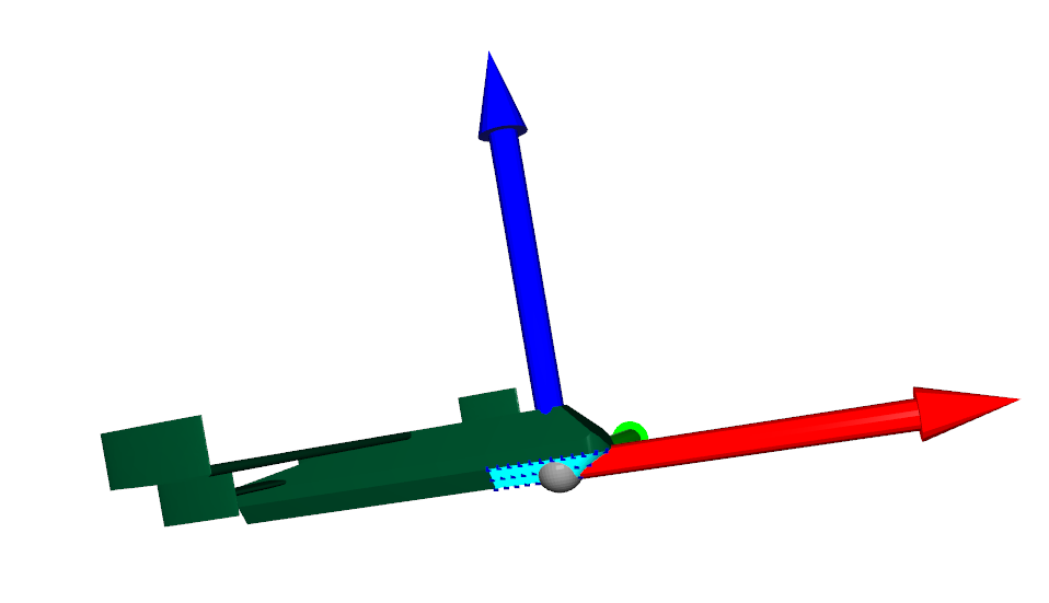
Visualise the Resultant UAV and Array

open3d.visualization.draw_geometries() can be used to visualise the open3d data structures open3d.geometry.PointCloud and open3d.geometry.PointCloud

mesh_frame = o3d.geometry.TriangleMesh.create_coordinate_frame(
    size=0.5, origin=[0, 0, 0]
)
o3d.visualization.draw_geometries([body, array, source_coords, mesh_frame])

# crop the inner surface of the array trianglemesh (not strictly required, as the UAV main body provides blocking to
# the hidden surfaces, but correctly an aperture will only have an outer face.
surface_array = copy.deepcopy(array)
surface_array.triangles = o3d.utility.Vector3iVector(
    np.asarray(array.triangles)[: len(array.triangles) // 2, :]
)
surface_array.triangle_normals = o3d.utility.Vector3dVector(
    np.asarray(array.triangle_normals)[: len(array.triangle_normals) // 2, :]
)

from lyceanem.base_classes import structures

blockers = structures([body, array])

from lyceanem.models.frequency_domain import calculate_farfield

from lyceanem.geometry.targets import source_cloud_from_shape

source_points, _ = source_cloud_from_shape(surface_array, wavelength * 0.5)

o3d.visualization.draw_geometries([body, array, source_points])

0.858793760075754
0.6307553291661078
0.3736530779617891
0.18721894988353757
0.034796457229518504
0.03058959422793881
-0.012054608990102791
0.02742812135247836
0.04455952883350341

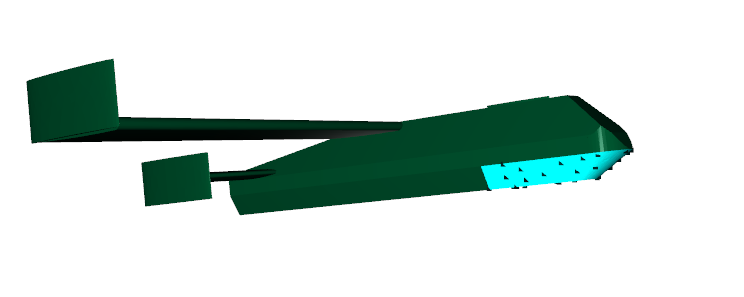
Drawbacks of lyceanem.geometry.geometryfunctions.sourcecloudfromshape()

As can be seen by comparing the two source point sets, lyceanem.geometry.geometryfunctions.sourcecloudfromshape() has a significant drawback when used for complex sharply curved antenna arrays, as the poisson disk sampling method does not produce consistently spaced results.

desired_E_axis = np.zeros((1, 3), dtype=np.float32)
desired_E_axis[0, 2] = 1.0

Etheta, Ephi = calculate_farfield(
    source_coords,
    blockers,
    desired_E_axis,
    az_range=np.linspace(-180, 180, az_res),
    el_range=np.linspace(-90, 90, elev_res),
    wavelength=wavelength,
    farfield_distance=20,
    project_vectors=True,
)

C:\Users\lycea\anaconda3\envs\cusignal-dev\lib\site-packages\numba\cuda\cudadrv\devicearray.py:885: NumbaPerformanceWarning: Host array used in CUDA kernel will incur copy overhead to/from device.
  warn(NumbaPerformanceWarning(msg))

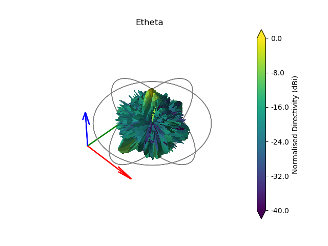
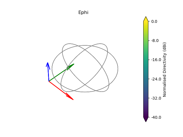
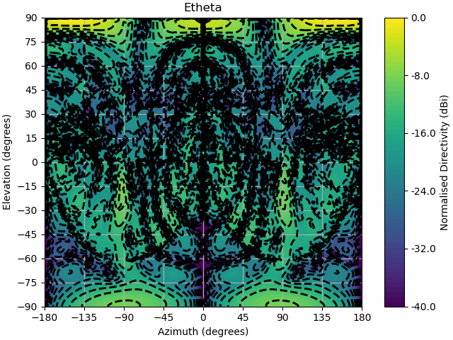
Storing and Manipulating Antenna Patterns

The resultant antenna pattern can be stored in lyceanem.base.antenna_pattern as it has been modelled as one distributed aperture, the advantage of this class is the integrated display, conversion and export functions. It is very simple to define, and save the pattern, and then display with a call to lyceanem.base.antenna_pattern.display_pattern(). This produces 3D polar plots which can be manipulated to give a better view of the whole pattern, but if contour plots are required, then this can also be produced by passing plottype=’Contour’ to the function.

from lyceanem.base_classes import antenna_pattern

UAV_Static_Pattern = antenna_pattern(
    azimuth_resolution=az_res, elevation_resolution=elev_res
)
UAV_Static_Pattern.pattern[:, :, 0] = Etheta
UAV_Static_Pattern.pattern[:, :, 0] = Ephi

UAV_Static_Pattern.display_pattern()

• 
• 

C:\Users\lycea\PycharmProjects\LyceanEM-Python\lyceanem\electromagnetics\beamforming.py:1170: RuntimeWarning: divide by zero encountered in log10
  logdata = 20 * np.log10(data)
C:\Users\lycea\PycharmProjects\LyceanEM-Python\lyceanem\electromagnetics\beamforming.py:1173: RuntimeWarning: invalid value encountered in subtract
  logdata -= np.nanmax(logdata)

UAV_Static_Pattern.display_pattern(plottype="Contour")

• 
• 

C:\Users\lycea\PycharmProjects\LyceanEM-Python\lyceanem\electromagnetics\beamforming.py:1170: RuntimeWarning: divide by zero encountered in log10
  logdata = 20 * np.log10(data)
C:\Users\lycea\PycharmProjects\LyceanEM-Python\lyceanem\electromagnetics\beamforming.py:1173: RuntimeWarning: invalid value encountered in subtract
  logdata -= np.nanmax(logdata)
C:\Users\lycea\anaconda3\envs\cusignal-dev\lib\site-packages\matplotlib\contour.py:1479: UserWarning: Warning: converting a masked element to nan.
  self.zmax = float(z.max())
C:\Users\lycea\anaconda3\envs\cusignal-dev\lib\site-packages\matplotlib\contour.py:1480: UserWarning: Warning: converting a masked element to nan.
  self.zmin = float(z.min())
C:\Users\lycea\PycharmProjects\LyceanEM-Python\lyceanem\electromagnetics\beamforming.py:1297: UserWarning: No contour levels were found within the data range.
  CS4 = ax.contour(